In this post we learn about DAX (Data Analysis Expressions) in Power BI. We will cover the basic concepts and fundamentals which can help us in implementing DAX in our reports.
At the end of this you should be able to:
1. Write DAX code to generate calculated columns, measures, and tables.
2. Understand intelligence functions and Quick measures to create complex DAX code.
What is DAX in Power BI?
DAX is a formula language used in Power BI and other Microsoft BI tools to perform data modeling and create custom calculations. It is based on the Excel formula language and provides a similar set of functions and operators for working with data in a Power BI dataset.
DAX can be used to define calculated columns in a Power BI table, create measures that perform calculations on the fly as you interact with the report, and filter and slice the data in a Power BI visualization. It is an essential tool for performing data analysis and creating dynamic, interactive reports in Power BI.
For simplicity we will split this entire lesson into three different posts:
1. Getting started with DAX
2. Context in DAX Formulas
3. Working with Date
Getting started with DAX
In DAX we have the concept of calculated columns and calculated measures. This concept is so important that we will spend good time understanding it before proceeding further. Let us begin by understanding the difference between the two.
Calculated Column Vs. Calculated Measures
In DAX, a calculated column is a column that you create in a table by defining a formula that performs a calculation on the data in that table. Calculated columns are similar to calculated fields in Excel, in that they allow you to perform calculations on the data in your Power BI dataset and display the results in a new column in the table.
Calculated columns are static, which means that the values in the column are calculated once when the table is loaded, and do not change as you interact with the report. Calculated columns are useful for performing calculations on the data in a table and storing the results for later use, such as in a visualization or as a filter.
On the other hand, a calculated measure is a measure that you create in DAX by defining a formula that performs a calculation on the data in your Power BI dataset. Calculated measures are similar to calculated fields in Excel, but they are more flexible and dynamic because they can be used to perform calculations on the fly as you interact with the report.
Calculated measures are useful for creating dynamic measures that change based on the filters, slicers, and other report interactions, such as calculating the average sales per customer for a given time period or the total sales for a specific product.
Points to remember
- In DAX columns evaluate at a row-level, therefore return one value per row and get stored in memory.
- However, measures evaluate at an aggregate-level, therefore return only one value and run at query time.
If you have understood the concept of calculated measures and calculated columns perfectly, you should have no difficulty in understanding why each card has been placed in the way it has been, if you still don’t understand it please go through the above theory once again before proceeding.

How to create calculated columns and measures in Power BI.
Here we will work with an example of Adventure Work Cycles who have just started their Power BI journey and want to understand their profitability.
We will create a column to see how much profit they gain from each order line in their sales table. To calculate profit, we will subtract the line cost from the line price.
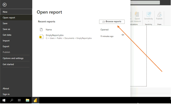
Step 1: We will open 1_1_profit_column.pbix from the Exercises folder
Click on files

Next, click on browse files

Now, open Excercises folder

Now open 1_1_profit_column.pbix file type to upload data.

Step 2: In this step we will rename the current Page 1 to “Profit”.
For this double click on Page 1 and rename it to “Profit”.


Step 3: Now we will create a new column in the Sales table called Profit that subtract line cost from line profit.
To do this we will go to the Data view while we are in the sales table. At the top menu, we have a button which says New Column.

Using the New Column we will solve for profit using the formula LineCost minus LinePrice.

Use the Name option to change the name of the column to profit.

Step 5: In the Report view, we will not create a Clustered column chart that shows the sum of Profit for each year.

Select the clustered column chart from the visualization field and drag orderdate and profit to x-axis and y-axis. Make sure the orderdata has year selected only and profit is sum. Using the above cluster chart we can answer how much profit Adventure Work Cycles made in 2016/2017/2018/2019.
Using Count Function
Let us proceed towards the next exercise.
Here, we will be utilizing a count function to understand the general trend of orders since Adventure Works started operating.
Step 1: We will begin by loading 1_2_sales_count.pbix from the Exercises folder.
Click on files

Next, click on browse files
Now, open Excercises folder

Now open 1_2_sales_count.pbix file type to upload data.

Step 2: We will create a new page in the report called “Sales Count”.
To do this on the Report view, next to the Profit page, click the + button which we can use to create a new report page – double click on the page and rename it “Sales Count”.

Step 3: We will now create a SalesCount measure in the _Calculations table which takes a discount Order Numbers.
To do this we will right click on _Calculations tables and select New Measure.

Next we will change the New Measure name to SalesCount and use the formula SalesCount = DISTINCTCOUNT(Sales[OrderNo])

Step 4: We will now create a line chat to the SalesCount by Order Date hierarchy. We will also use the chart drill-down feature to “Expand all down one level in hierarchy: twice to see Month Year view.
To do this we will begin by selecting a line chart, drag OrderDate on x-axis and SalesCount on Y-axis. In the Canvas we will use the drill button to arrive at a month data and using this graph we can find the month year in which largest number of orders arrived.

Calculating Profit margin ratio
We will now create a measure to represent the profit margin ratio, thus we will compare the total profit to the total sales.
Here, in the Exercise we have been TotalSales and we have calculated the Profit column above, now we will use it to arrive at Total Profit.
Let us start working.
Step 1: We will begin by creating a new page in the report called “Profit Margin Ratio”.

Step 2: Now we will create a Total Profit measure inside the _Calculations table, this will be the sum of all the profit columns. We will use the formula
Total Profit = Sum(Sales[Profit]) here.

Step 3: Now we will create a measure called ProfitMarginRatio in the _Calculations table which we can obtain by dividing Total Profit by Total Sales. We will also Format ProfitMarginRatio so that it displays as % with two decimal points.
We will use the formula = ProfitMarginRatio = ‘_Calculations'[Total Profit] / ‘_Calculations'[Total Sales]
Step 4: Here we will select the line chart to visualize the ProfitMarginRatio by Order Year.

Here we are 🙂
We have learned how to get started with DAX in Power BI. Next we should learn about Context in DAX.